Thursday, 19 March 2015

Creating Graphical Indicator Fields in Microsoft Project


Graphical indicator fields can be used to make it easier for people viewing the project plan, to know the status of a numerical field. Instead of displaying the value, a coloured icon is used as an indicator.

By using graphical indicators, a field’s status can easily be viewed at a glance, in much the same way that Conditional Formatting is used on an Excel spreadsheet.

Values or graphical indicators


In this article, graphical indicators have been used to display cost variance (as shown in the image above). If we have overspent on a task then a red unhappy face is displayed, yet if we are on budget then a green happy face is shown.

Creating the Custom Field


The first step is to create the custom field. In this example, we want to create a custom field for the cost variance value.

There is already a field for cost variance, but we want to create an additional one to the one that exists for the graphical indicator.

  1. When in Gantt Chart view, click the Format tab on the Ribbon and then Custom Fields.

Completed custom fields dialog box


  1. Click the Type list in the top right corner and select Cost as the field type. You can see that there are many other types you could use such as text, number and date.
  2. Click Rename and enter a name for this new custom field. The name On/Over Budget has been used in this article.
  3. Click the Formula button. We need to get this field to display the information from the Cost Variance field. Click the Fields button, then Cost and then Cost Variance.
Formula to display cost variance data


Displaying the Graphical Indicators


Now we have our custom field, we need to set it to display the graphical indicators instead of the cost variance value.

  1. Click the Graphical Indicators button.
  2. We need to set the criteria for them. Enter the criteria as displayed in the image below. Choose your own choice of indicator from the Image column.

Setting the criteria for the graphical indicators
 

  1. Click Ok to close both the Graphical Indicators and Custom Fields dialog.

Inserting the Column


Now that the field has been created, you need to insert it into the table.

  1. Right click the column header to the right of where you want the field to appear in the table.
  2. Select Insert Column and find the field in the list by beginning to type its name. In this example it is On/Over Budget.

Graphical Indicators displayed on table


The graphical indicators are displayed in the column. Position your mouse pointer over the field to see the value.

Showing the cost variance as a value


Watch the Video


More Microsoft Project Tutorials

Sunday, 2 November 2014

5 Advanced Lookup Formula Techniques


Lookup functions such as VLOOKUP are some of the most commonly used functions in Excel. They are used to achieve many different Excel tasks.

If you are reading this blog post you have probably used VLOOKUP or one of the other lookup functions before. This article looks at 5 advanced lookup techniques.

Monday, 4 August 2014

The Pie of Pie Chart in Excel Demystified

Pie charts are used to display data points as a percentage of the whole value. Excel provides a few different variations of pie chart to choose from. One with a difference is the pie of pie chart.

The pie of pie chart is used to display the smaller values of a pie chart in a secondary pie to make them more visible.

Take the pie chart below for instance. The loyalty coupon, offline and referrals values make up such a small percentage of the pie chart that they are difficult to read and understand.

Pie chart struggling to handle minor values


Let’s see the same data set using a pie of pie chart. The primary pie displays the smaller values making up 5% of the whole value. These values are then displayed in a secondary pie giving much more attention to the detail.

The smaller data points retain their percentages as a contribution to the whole and lines are used to visualise the enhanced segment easily.

Pie of Pie chart in Excel

Sunday, 13 July 2014

Create Conditional Hyperlinks in Excel

Take your hyperlinks to another level with the HYPERLINK function. This function can be used to create conditional hyperlinks that only display when required. The hyperlinks are also dynamic and can change their link location or anchor text automatically.

In this blog post we will look at both of these techniques.

Monday, 30 June 2014

Forecasting Future Values in Excel

While Excel is not able to predict the future, it is a capable of forecasting future values using existing data.

Excel provides many functions that are capable of predicting future values that reflect past data. These different functions cater for the different ways that your data may be plotted. For example, if your data has a steady growth or if it fluctuates dramatically.

They include FORECAST, TREND, LINEST and GROWTH to name a few.

However in this tutorial we will focus our attention on adding a trendline to a chart to forecast future values.

Adding a Trendline to a Chart


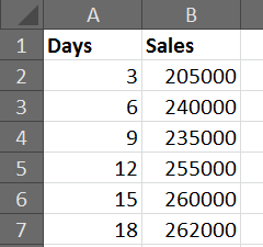
For this example we will be using the sales data displayed below. We would like to forecast the sales for the next 3 periods (9 days) based on the sales from the previous 6 periods (18 days).

Previous sales data


Click the Layout tab on the Ribbon and then Trendline (This option has changed a little over time. This example is for Excel 2007 and 2010).

Select More Trendline Options.

Add a trendline to a chart


There are 6 different types of trendline to choose from for your chart. The list below explains how you can decide which one is best for your data.

Linear – Used for values that increase or decrease at a steady rate.

Logarithmic – Used for values that increase or decrease quickly before levelling out.

Polynomial – Used for values that fluctuate.

Power – Used for values that increase or decrease at a specific rate.

Exponential – Used for values that increase or decrease at increasingly higher rates.

Moving Average – Averages out the high and low points smoothing any fluctuations.

Select the trendline that best suits your data from the options provided.

In the Forecast Forward field, enter the number of periods in the future that you wish the trendline to display for.

Before we add the trendline, another useful option in this dialog box is the Display R-squared value on chart checkbox. The R-squared value represents the accuracy of the trendline.

This value is a number between 0 and 1. The closer to 1 that the value is, the more accurate the trendline.

The image below shows a linear trendline added to the chart. It has an R-squared value of 0.8236, which is fairly accurate.

Excel chart with a linear trendline


However our sales appear to be levelling out.

The image below shows a logarithmic trendline being used on the chart instead. An R-squared value of 0.9186 indicate that this trendline is a better reflection on the past data.

Logarithmic trendline that better reflects sales data


Watch the Video


Tuesday, 17 June 2014

Calculate a Future Date in Excel

When working in Excel you may need to calculate a future date. This may be for example, when somebody’s work probation period ends, or the date a rented car should be returned.


In this article we explore a few different techniques for calculating the future date. These include how to exclude certain dates such as weekends and holidays.

Saturday, 7 June 2014

Return the Cell Reference instead of the Value from a Lookup

In Excel, Lookup functions such as Vlookup or Index and Match can be used to find a record and return a value. But what if you want to return the cell reference, or address, instead of the value.

In this example we will look for a Customer using its ID and return the address of the cell that contains the customer’s city.


Monday, 2 June 2014

Fixing Formula Errors

Working with formulas is the building block of creating powerful and dynamic Excel spreadsheets. However when there is a problem, it is not always that easy to diagnose what the problem with your formulas is.
Fortunately there a few tools provided with Excel to assist you in fixing formula errors on your spreadsheet.
 

Formula Error Messages

 
When an error occurs you will be shown an error message.
 
Formula error messages begin with a number sign (#) and are then followed by some text that gives an indication as to the type of problem you encountered.
 
Understanding these error messages can help you solve your formula problems.
 
Some common formula error messages include;
  • #NAME? – Excel does not recognise the text you entered as a reference to a range, table or function.
  • #REF! – Excel cannot find the cell that you referenced within the formula.
  • #VALUE! – Normally a formatting issue. For example, a cell your formula is referencing may contain text instead of a number.
  • #DIV/0! – Occurs when you try and divide by 0 or an empty cell.
  • #NUM! – Normally occurs when you try and pass invalid data to an argument like text rather than a number.
  • ######## - Either the number is too large for the cell that is displaying it, or it contains a date before 01/01/1900.

Tracing Precedents and Dependents


When trying to trace the cause of a formula error, the Trace Precedents and Trace Dependents buttons will illustrate the cells that the formula is dependent on (precedents), and those affected by the formula result (dependents).
 
These buttons can be found on the Formulas tab of the Ribbon.
 
The image below shows the Trace Precedents button identifying the cells that the formula in B17 is dependent upon. It highlights that the issue is caused by the contents of cell B5.

Trace precedents of a formula
  

Displaying Formulas
 

By default Excel displays the value (or formula result) in a cell and the formula in the Formula Bar. This means that you need to select a cell to view the underlying formula.
 
If you are trying to diagnose a large formula that references other cells (which may also contain formulas), this can get irritating.

Fortunately you can toggle the display of formulas on and off. Making them visible in the cell can make them easier to troubleshoot.
 
Click the Formulas tab on the Ribbon, and then Show Formulas in the Formula Auditing group.
 

Show Calculation Steps and Error Checking


When a formula is quite large you may have trouble locating where the error is occurring.
 
Good news is that Excel will show you the calculation steps of the formula. This means that it will run the formula and stop at the point just prior to the error occurring. It even underlines the problem part.

Click the smart tag icon next to the cell containing the error, and select Show Calculation Steps from the menu.

Error checking options for a formula
 
Excel steps through the formula, displaying the values used and stops when it cannot go any further without producing the error.

Show calculation steps to find source of error

This example highlights that the issue was that a cell contained text. A basic example but it demonstrated using these features to find the fault.
 
Let’s look at a stronger example. There is an error in the formula below.

#REF error in large formula
 
Click the Error Checking button on the Formulas tab. This provides an explanation of the suspected problem. It mentions that a cell may have moved, or that a function is returning a reference error.

Error Checking dialog box with explanation of problem
 
Click the Show Calculation Steps button to step into the formula. The first Vlookup function is underlined highlighting the problem function.

Evaluate formula highlighting the problem area
 
You now have the source of the problem from a formula that used 4 different functions. Click the Evaluate button to see the error occur.

Formula error caused by the Vlookup function
 
The actual problem with this formula is that we have asked to return data from column 11, but the table array for the Vlookup is only 10 columns wide.
 
Boost your Excel formula skills to superhero status, sign up for our Excel Superhero course.

More Tips for Troubleshooting Formula Errors


Saturday, 3 May 2014

5 Awesome Excel 2013 Flash Fill Examples


Flash Fill is one of the biggest new features to be released with Excel 2013. In fact let me re-phrase that. Flash Fill is one of the biggest new features to ever be released with Excel.

It can do so much with your data, the first time I saw its true power it nearly knocked me off my chair.

It can be used to extract text and values from a cell, concatenate data, change its case and even reverse data.

How to use Flash Fill in Excel 2013


Probably the best thing about this powerful new tool is how easy it is to use.

To use Flash Fill;

  1. Click in a cell and type in an example of how you want your data to look.
  2. Press the Ctrl + E keys, or select the range of cells including the example and press the Flash Fill button on the Data tab.

Tuesday, 22 April 2014

Understanding Section Breaks in Microsoft Word

Section breaks are one of the most useful features of Microsoft Word, especially when working with long documents.

They enable you to apply page formatting to parts of a page, or to specific pages of a document.
This article will look at two awesome uses of section breaks in Microsoft Word.

First we look at using them to insert a landscape page in the middle of a portrait orientated document. We then look at using them to start page numbering in a document from a specific page.


Saturday, 8 February 2014

Calculate Median and Mode Using Multiple Conditions

This tutorial looks at how you can create conditional median and mode formulas.

When calculating averages based on multiple conditions, Excel provides a function called AVERAGEIFS. This is great for calculating the mean of a set of numbers. However they do not provide an equivalent for calculating the median and mode using multiple conditions.

To achieve this we will need to create an array formula by nesting the IF function within the median and mode functions.

For this example we will be using a list of real estate prices.


Real estate prices


Conditional Median Formula

The MEDIAN function is used to calculate the middle value from a set of values. The formula below, entered in cell H3, calculates the median real estate price for a specific town.

Conditional median formula


Monday, 7 October 2013

Create an Excel Soccer League Table Generator


Need a league table generator for a sports league you compete in or manage?

I love sport and Excel to merge the two is enjoyable for me. I have created a league table generator in Excel so that when results are entered for a fixture, the league table will calculate and rank each team accordingly.

Excel soccer league table generator


You don't need to do a thing. After setup just enter the results and let the league table take care of the rest.

Download the Excel league table generator

To use the spreadsheet;
  1. Enter the team names onto the Teams sheet
  2. Enter the fixtures onto the fixtures sheet (check out my Excel fixture list creator)
  3. Enter the results as they happen
Check out the Create sports league tables and tournament in Excel online course and learn how you can set up your own league tables now.
 

Friday, 9 August 2013

Calculate Length of Service in Excel

If you are using Excel to store data about employees in a company, you may at some point need to calculate their length of service. Let’s say we want to return how many years and months an employee has worked for our company.

The DATEDIF function in Excel is used to calculate the difference between two dates. The difference can be returned as the number of years, months or days.

As we wish to return the number of years and months that they have worked we will concatenate two DATEDIF functions together.

Monday, 5 August 2013

Excel VBA: List All the Excel Files in a folder

Using Excel VBA you can get a list of all the files in a folder and enter them on a worksheet. We can also retrieve certain information about the file if required. This macro will list the file names and the date they were last modified.

How does it Work?

The folder picker dialog box is used to make it easier for the user to select the folder they want to return files from. An If statement has been included to ensure that the user did select a folder.
The Dir function will be used to return each filename from the folder or directory. This function will then be used to iterate through each file in turn (Learn more about the Dir function in Excel VBA).
The macro in this tutorial will list all Excel files in a folder to the worksheet. This has been specified by using *.xls in the Dir function. The wildcard and extension can be altered to list the files you want, or omitted entirely to list all files in the folder.
The FileDateTime method has been used to capture the date the files were last created or modified.

Thursday, 1 August 2013

Check for Odd Numbers in Excel

Data accuracy is essential in Excel. If data entered is incorrect then your skills with PivotTables and Filtering data become almost irrelevant.

In this post we look at preventing the entry of odd numbers in a range, or just highlighting them for further interrogation.

Thursday, 25 July 2013

Use Comments for Storing Large Amounts of Text

Excel was built to handle records of data that contain labels, values and formulas. Storing large amounts of text is not its priority meaning your spreadsheets can become long, wide and awkward.

Typically to accommodate bulk text columns such as for descriptions and notes you will make the column wider, apply wrap text to the cells, or a bit of both. These features can help, but another option available to you is to store the text in a comment.

By storing the text in a comment box it is only visible when you want it. By not storing it in a cell your spreadsheet remains easy to navigate and use daily.

Thursday, 18 July 2013

Netball League Table Generator in Excel

I recently helped a reader out by creating a netball league table generator in Excel.

She wanted to be able to enter the results onto a sheet and have the league table automatically update to rank teams appropriately.

The spreadsheet allows 5 points for a win and 3 for a draw. 1 point is earned if the losing team scores half the points of the winning team. It also provides the ability deduct penalty points from a team.

Monday, 17 June 2013

Import Data from the Web into Excel

You can import data from the web into Excel for analysis and reporting. When data is imported from the Internet, a connection is established. This means that the link can be updated, and you will not have to repeat this import process every time the data is needed.

For this example, we will look at importing data from www.soccerstats.com. This is a favourite site of mine. It contains up to date statistics from soccer leagues all over the world. We will import the La Liga top scorers table.

Thursday, 2 May 2013

Excel VBA: The Dir Function


In Microsoft Excel VBA, the Dir function is used to return the first filename from a specified directory, and list of attributes. The filename is returned as a string.
The Dir function can then be entered without any arguments to return the next filename from that directory.
The most common use of the Dir function is to loop through all the files in a folder to perform an action on each one. Other common uses include checking if a file or a directory exists, or to look for a specific file such as the latest one.

Dir Function Syntax

When entering the Dir function into the Visual Basic Editor the quick info list should appear and prompt for the following.
Dir( [PathName], [Attributes As VbFileAttribute = vbNormal]) As String

Thursday, 25 April 2013

Create a Speedometer Chart in Excel


Speedometer charts are used to measure performance. As a speedometer can be found on any car dashboard they are instantly recognisable, and will add a certain style to your Excel dashboards.
Excel does not provide one as a default chart type, so to create a speedometer chart in Excel we will need a donut chart, a pie chart and a little ingenuity.
The Donut chart will be used for the speedometer background and the Pie chart will be positioned on top to create the needle.
Being a big fan of the UFC, I thought I would create a speedometer chart to display the percentage of victories by UFC Welterweight champion Georges St. Pierre that have come via by stoppage (submission, KO or TKO).
Create a speedometer chart in Excel


.