
Lookup functions such as VLOOKUP are some of the most
commonly used functions in Excel. They are used to achieve many different Excel
tasks.
If you are reading this blog post you have probably used
VLOOKUP or one of the other lookup functions before. This article looks at 5
advanced lookup techniques.
Lookup a Value using Multiple Conditions
Lookup functions are used to look for a value using single
criteria. However, you can create lookup functions to search using multiple
conditions.
In the image below a formula has been entered to return the
value where the department is Training
and the Region is India.
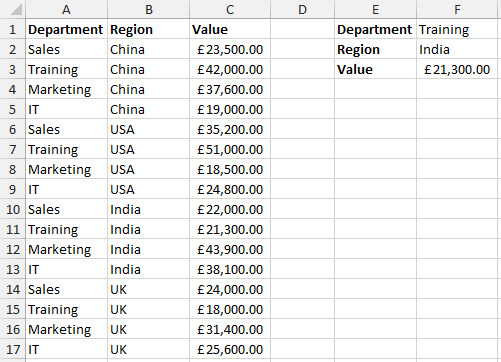
The formula below has been used to create this lookup using
multiple conditions. This is an array formula so you need to press Ctrl + Shift
+ Enter to run the formula. Do not type the curly braces manually. They appear
when the formula is entered.
{=INDEX(C2:C17,MATCH(1,(A2:A17=F1)*(B2:B17=F2),0))}
Use VLOOKUP to Look Across Multiple Sheets
What if you need a VLOOKUP function to look for a value in
more than one table? Well fear not because you can get your VLOOKUP to check
across multiple sheets, or tables, for a value.
The formula below uses the IFERROR function to get VLOOKUP
to look in another table if it cannot find the value. This formula searches
across 3 different tables for an Employee ID.
If the employee cannot be found then the text “Not found” is
returned.
=IFERROR(VLOOKUP(A2,Region1!A1:B4,2,false),IFERROR(VLOOKUP(A2,Region2!A1:B4,2,false),IFERROR(VLOOKUP(A2,Region3!A1:B4,2,false),”Not
found”)))
Lookup a Picture in a List
Lookup functions are normally used to return a value, but
they can also be used to look for and return a picture. To create a picture
lookup you cannot write a lookup function in a cell the way that you would to
return a value.
You will need to create a defined name and write the lookup
function as its reference. The picture you want to return is then linked to the
defined name.
Watch the video below to see how to create a picture lookup.
In this example the picture of a flag is returned dependent upon what country
is selected from a list.
Compare Two Lists for Missing Records
A popular use of lookup functions is to compare two lists. For
example, you may want to compare one list with another and highlight the
missing items.
In this example the MATCH function is combined with
Conditional Formatting to highlight the rows of the missing records.
- Select the table excluding the headings (the whole table is selected so that the entire row is highlighted).
- Click the Home tab and then Conditional Formatting.
- Select New Rule and then Use a Formula to determine which cells to format.
- Enter the formula below into the box provided and choose the formatting you wish to apply.
=ISNA(MATCH($A2,$F$2:$F$19,0))
The MATCH function looks for a value in column A (beginning
with A2 as the first row of data). It looks for the value in another table that
begins from column F.
If the MATCH function cannot find the value then the #N/A
error is returned. The ISNA function is used to detect this and get Conditional
Formatting to change the colour of the cells in response.
Return the Address of a Value
You may need to return the cell address of a value in a
range. You can determine the cell address by using the ADDRESS function with
the MATCH function.
The image below shows a snapshot of a list of customers. Let’s
say you wanted to return the cell address of the city for the customer you are
looking for in this list.

The formula below can be used to achieve this where cell A2
contains the customer ID you are looking for, and the number 5 specifies the
column you want to return (column E).
=ADDRESS(MATCH(A2,Customers!A:A,0),5)
By default, the cell address is returned as an absolute cell
reference. There are extra optional arguments to the ADDRESS function allowing
you to specify the type of cell address (relative or absolute), and also to
include a sheet name in the address.
The Lookup and Reference functions of Excel are an
incredibly powerful and useful category of functions. They are used heavily in large
spreadsheets to automatically return data and dynamically link different
sheets.
This article covers 5 advanced lookup techniques. These functions
have a lot to offer an Excel user.
No comments:
Post a Comment