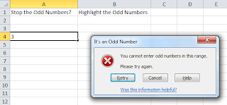
In this post we look at preventing the entry of odd numbers
in a range, or just highlighting them for further interrogation.
Prevent Odd Numbers in a Range
To prevent the entry of odd numbers in a range we will need
Data Validation. We will also need a formula to identify the odd numbers.
The formula we will use is the MOD function. This function
returns a remainder when a number is divided by a divisor.
For us this means that if we divide the number in the cell
we are checking by 2, and the remainder is 0 then the number is even, and if it
returns 1 then the number is odd.
1. Select the
range you want to apply the Data Validation rule to.
2. Click the Data tab on the Ribbon and then the
Data Validation button.
3. Select Custom from the Allow drop list. We need
to use custom as we are entering a formula.
4. In the Formula box enter =MOD($A2,2)=0. Replace
$A2 with the first cell of the range you are validating i.e. if you selected
column C in step 1 then use $C1 in your formula.
5. Click the Error Alert tab. We will create a
customised error message so that users know that entering odd numbers is wrong.
6. Click in the Title box and enter a title for
your message box, then enter your message in the Error message box.
7. Click Ok and your validation is set and ready to
go.
Try entering an odd number to see your error
alert returned, then try and even number to check that it is accepted.
Watch the Video
Highlight the Odd Numbers in a List
Instead of preventing the entry of odd numbers, you may wish
to highlight them. You can then work with the odd numbers by sorting and filtering.
For this task we will combine the Conditional Formatting
tool with the ISODD function. The ISODD function will return true if the number
is odd.
1. Select the range of cells that you want to
format.
2. Click the Home tab on the Ribbon and the Conditional
Formatting button.
3. Select New Rule from the list.
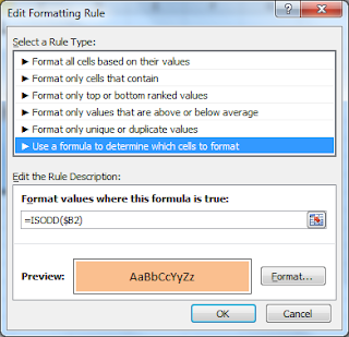
4. Select Use a formula to determine which cells to
format.
5. Enter the formula =ISODD($B2) in the box
provided. Replace $B2 in the formula with the first cell in the range of cells
you selected in step 1.
6. Click the Format button and choose the
formatting you wish to apply.
7. Click Ok to close down all boxes and the odd
numbers in your range should be highlighted.


No comments:
Post a Comment